TensorFlow Lite实践：ESP32 + 红外传感器实现火焰检测

一、介绍

在嵌入式设备上实现智能识别任务，一直面临着资源受限和部署复杂的挑战。幸运的是，TensorFlow Lite for Microcontrollers（TFLM） 提供了一套轻量化、可在无操作系统和少量内存环境下运行的机器学习框架，使我们可以在像 ESP32 这样的微控制器上运行神经网络模型。

使用 TensorFlow Lite Micro 的优势：

• 轻量化部署：模型经过量化和转换后，大小通常在几十 KB，适配资源紧张的 MCU。
• 无需操作系统：TFLM 设计为裸机环境运行，无需 RTOS 支持。
• 开源可裁剪：源码完全开源，可根据需求裁剪只用到的算子，降低代码体积。
• 跨平台适配性强：可运行于 Arduino、ESP-IDF、Zephyr 等多种嵌入式平台。
• 系统总体设计思路（传感器 + 模型推理 + 结果响应）

系统总体设计思路：

项目以 红外传感器（ MLX90640） 采集热数据，通过部署在 ESP32 上的神经网络模型，实现对 火焰状态的分类检测。系统主要由以下几个模块组成：

1. 数据采集模块：使用红外传感器定时采集热图或温度数据，数据格式为2D 热图（取决于传感器）
2. 模型推理模块：将采集的数据输入 TFLite 模型（嵌入在固件中），输出为分类结果，例如 “有火焰” / “无火焰”
3. 结果响应模块：据推理结果进行相应动作：蜂鸣器报警/LED 指示/串口打印状态/MQTT 上传云平台

二、硬件与软件准备

2.1 硬件列表

为了在资源有限的设备上实现红外图像识别和火焰检测，本项目选用了性价比极高的 ESP32-C3 开发板(特地没有使用高性能的S3)搭配红外热成像模块和显示组件：

组件	说明
ESP32-C3 开发板	低功耗、RISC-V 架构，带 WiFi 支持，适合边缘计算部署
MLX90640 红外热成像传感器	支持 32×24 热像素阵列，I²C 通信，测温范围广，适合获取热图
TFT 屏幕（ST7789 240×240）	实时显示热图或识别状态，增强交互性
LED 指示灯	用于识别结果的本地报警提示
供电模块（如锂电池、Type-C 转 5V）	提供稳定供电，支持便携部署

2.2 软件工具

为了完成从数据采集、模型训练、模型转换到最终部署，需要准备以下软件环境：

工具	用途说明
Arduino IDE / PlatformIO	用于编写和烧录 ESP32-C3 上的推理逻辑与外设驱动
Python + TensorFlow	用于模型构建、训练、量化与 TFLite 转换
TensorFlow Lite 转换工具	将 .h5 或 .pb 模型转换为 .tflite 并量化压缩
xxd 工具	将 .tflite 文件转换为 C 数组，用于嵌入固件中

三、传感器数据采集与分析

为了训练一个可以判断火焰状态的模型，首先需要获取可靠的红外热成像数据，并将其转化为可用于训练的标准数据集。本节将介绍数据采集、标注与分析的基本流程。

如何读取红外传感器数据

本项目使用 MLX90640 红外热成像传感器，它可以提供一个 32×24 的热图像矩阵，每个像素代表一个温度值。通过 I²C 接口读取原始帧数据，并进行处理，可得到一张包含 768 个温度点的热图。

示例代码展示如下：

/*********************************************************
  MLX90640-D55 数据收集测试程序（CSV输出，带标签）
*********************************************************/
#include <Wire.h>
#include <Adafruit_MLX90640.h>

/*========== 参数配置 ==========*/
#define LABEL 1 // 数据标签：0 = 无火焰，1 = 有火焰

constexpr uint8_t SDA_PIN = 11;
constexpr uint8_t SCL_PIN = 10;
constexpr uint8_t MLX_ADDR = 0x33;
constexpr uint32_t I2C_HZ = 100000;
constexpr mlx90640_refreshrate_t FPS = MLX90640_2_HZ;
/*=============================*/

Adafruit_MLX90640 mlx;
float frame[32 * 24];
bool headerPrinted = false;

void setup()
{
  Serial.begin(115200);
  delay(50);

  Wire.begin(SDA_PIN, SCL_PIN);
  Wire.setClock(I2C_HZ);

  Serial.println(F("\nMLX90640-D55 init…"));
  if (!mlx.begin(MLX_ADDR, &Wire))
  {
    Serial.println(F("ERROR: 传感器未找到！"));
    while (true)
      delay(1000);
  }

  mlx.setMode(MLX90640_CHESS);
  mlx.setResolution(MLX90640_ADC_18BIT);
  mlx.setRefreshRate(FPS);

  Serial.println(F("初始化完成，开始采集…"));
}

void loop()
{
  if (mlx.getFrame(frame) != 0)
  {
    Serial.println(F("读取失败，跳过本帧"));
    delay(10);
    return;
  }

  // 打印 CSV 表头（只打印一次）
  if (!headerPrinted)
  {
    Serial.print("label");
    for (int i = 0; i < 768; i++)
    {
      Serial.print(",p");
      Serial.print(i);
    }
    Serial.println();
    headerPrinted = true;
  }

  // 打印一帧数据（第一列为标签）
  Serial.print(LABEL);
  for (int i = 0; i < 768; i++)
  {
    Serial.print(",");
    Serial.print(frame[i], 2); // 保留 2 位小数
  }
  Serial.println();

  delay(1000); // 控制采样频率（每秒采一帧）
}

代码串口格式输出如下，我们只需要只需修改#define LABEL 0/1来切换采集状态。

label,p0,p1,p2,...,p767
1,26.38,26.41,26.42,...,45.23
1,26.37,26.39,26.40,...,45.18
...

并且我们可以通过一个配套的 Python 脚本，用于收集串口数据直接存成 CSV 文件：

import serial
import csv
import time

# ============ 参数配置 =============
PORT = 'COM3'           # 串口号（Windows示例）Linux可用 '/dev/ttyUSB0'
BAUD = 115200           # 波特率
OUTPUT_CSV = 'mlx90640_data.csv'
MAX_SAMPLES = 100       # 采集帧数上限（设为 None 无限采集）
SHOW_PROGRESS = True    # 是否打印实时信息
# ===================================

def main():
    ser = serial.Serial(PORT, BAUD, timeout=2)
    time.sleep(2)  # 等待串口稳定

    print(f"连接到 {PORT}，开始采集…")
    with open(OUTPUT_CSV, 'w', newline='') as f:
        writer = csv.writer(f)
        sample_count = 0
        header_written = False

        while True:
            try:
                line = ser.readline().decode('utf-8').strip()
                if not line:
                    continue

                row = line.split(',')

                # 写入表头（首行为 label,p0,p1,...）
                if not header_written and row[0] == 'label':
                    writer.writerow(row)
                    header_written = True
                    continue

                # 跳过尚未开始输出的数据
                if not header_written:
                    continue

                # 写入数据行
                writer.writerow(row)
                sample_count += 1

                if SHOW_PROGRESS:
                    print(f"采集第 {sample_count} 帧")

                # 是否达到上限
                if MAX_SAMPLES and sample_count >= MAX_SAMPLES:
                    print(f"已采集 {sample_count} 帧，保存至 {OUTPUT_CSV}")
                    break

            except KeyboardInterrupt:
                print("\n手动中止，保存数据")
                break
            except Exception as e:
                print(f"异常：{e}")
                continue

    ser.close()
    print("串口关闭，采集完成。")

if __name__ == '__main__':
    main()

采集到的数据如下：

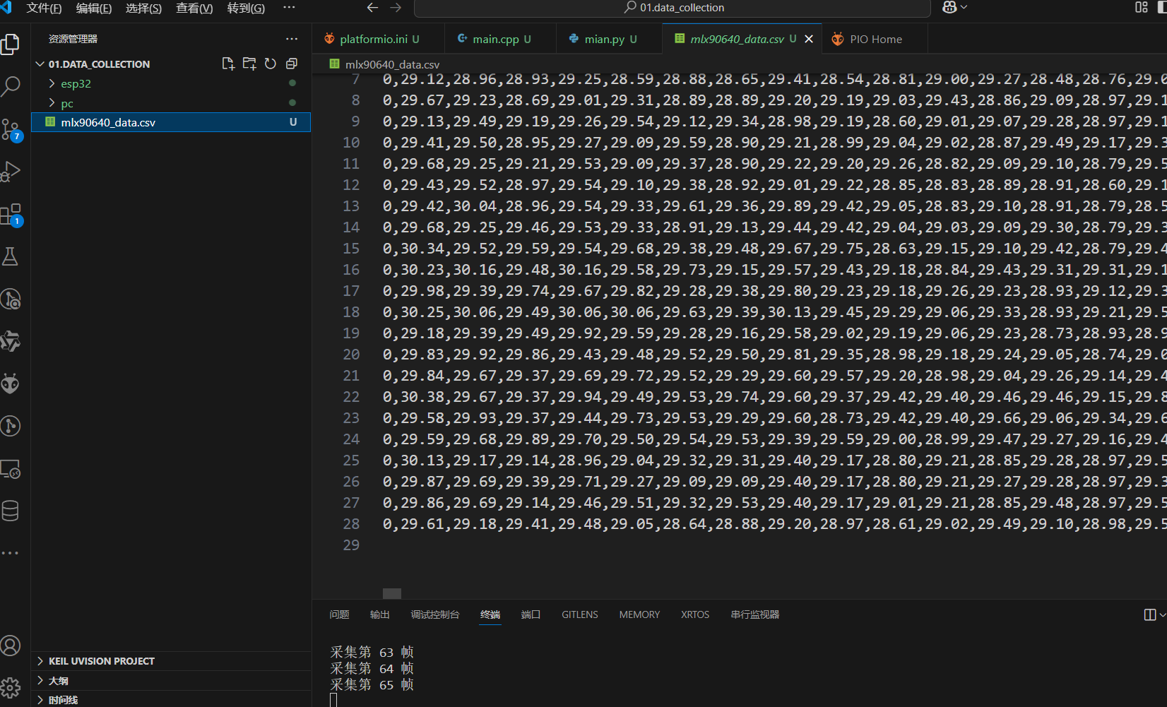
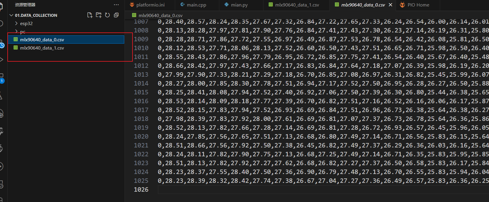
我们只需要分别采集不同情况的数据即可（这里每种数据采集1024个）。

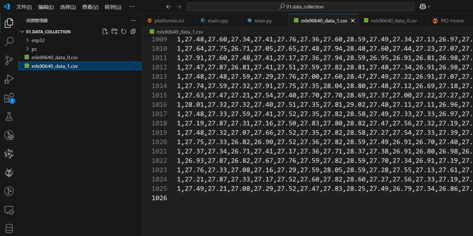
最终我们成功驱动有火源和无火源两种情况下的数据样本，各自1024个:

简单的数据可视化与初步观察（可选）：

我们可以简单的使用下面的脚本来预览我们采集到的数据：

import pandas as pd
import matplotlib.pyplot as plt
import numpy as np
import seaborn as sns
from mpl_toolkits.axes_grid1 import make_axes_locatable

# 加载数据文件
data_fire = pd.read_csv('data/mlx90640_data_1.csv')  # 有火源数据
data_no_fire = pd.read_csv('data/mlx90640_data_0.csv')  # 无火源数据

# 提取特征（温度数据）和标签，确保转换为浮点数
features_fire = data_fire.iloc[:, 1:].astype(float).values  # 有火源数据的温度值
features_no_fire = data_no_fire.iloc[:, 1:].astype(float).values  # 无火源数据的温度值

# 计算基本统计信息
print("有火源数据统计信息：")
print(f"样本数量: {len(features_fire)}")
print(f"平均温度: {np.mean(features_fire):.2f}°C")
print(f"最高温度: {np.max(features_fire):.2f}°C")
print(f"最低温度: {np.min(features_fire):.2f}°C")
print(f"温度标准差: {np.std(features_fire):.2f}°C")
print("\n无火源数据统计信息：")
print(f"样本数量: {len(features_no_fire)}")
print(f"平均温度: {np.mean(features_no_fire):.2f}°C")
print(f"最高温度: {np.max(features_no_fire):.2f}°C")
print(f"最低温度: {np.min(features_no_fire):.2f}°C")
print(f"温度标准差: {np.std(features_no_fire):.2f}°C")

# 设置matplotlib中文字体
plt.rcParams['font.sans-serif'] = ['SimHei']  # 用来正常显示中文标签
plt.rcParams['axes.unicode_minus'] = False  # 用来正常显示负号

# 创建一个函数来绘制热力图
def plot_thermal_image(data, title, subplot_pos):
    plt.subplot(subplot_pos)
    im = plt.imshow(data.reshape(24, 32), cmap='coolwarm', interpolation='nearest', vmin=0, vmax=120)
    plt.title(title)
    divider = make_axes_locatable(plt.gca())
    cax = divider.append_axes("right", size="5%", pad=0.05)
    plt.colorbar(im, cax=cax, label='温度 (°C)')

# 创建一个大的图形来包含随机样本子图
plt.figure(figsize=(20, 10))

# 随机选择4个样本索引
random_indices = np.random.choice(len(features_fire), 4, replace=False)

# 热力图对比（随机样本）
for i, idx in enumerate(random_indices):
    # 有火源样本
    plt.subplot(2, 4, i+1)
    im = plt.imshow(features_fire[idx].reshape(24, 32), cmap='coolwarm', interpolation='nearest', vmin=0, vmax=120)
    plt.title(f'有火源样本 {idx+1}')
    plt.colorbar(label='温度 (°C)')
    
    # 无火源样本
    plt.subplot(2, 4, i+5)
    im = plt.imshow(features_no_fire[idx].reshape(24, 32), cmap='coolwarm', interpolation='nearest', vmin=0, vmax=120)
    plt.title(f'无火源样本 {idx+1}')
    plt.colorbar(label='温度 (°C)')

plt.tight_layout()
plt.show()

# 在新的图形中显示平均热力图
plt.figure(figsize=(15, 5))
# 有火源平均热力图
plot_thermal_image(np.mean(features_fire, axis=0), '有火源平均热力图', 121)
# 无火源平均热力图
plot_thermal_image(np.mean(features_no_fire, axis=0), '无火源平均热力图', 122)
plt.tight_layout()
plt.show()

显示效果如下：

样本对比：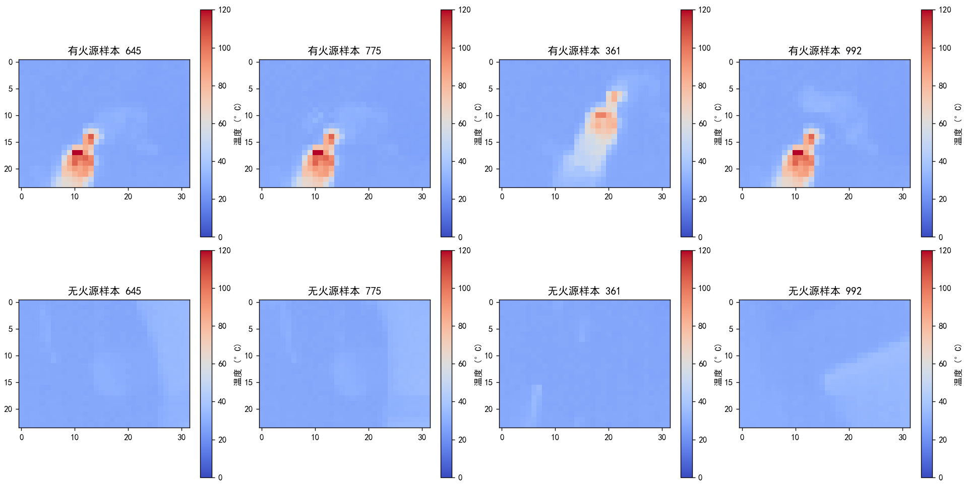

均值对比：

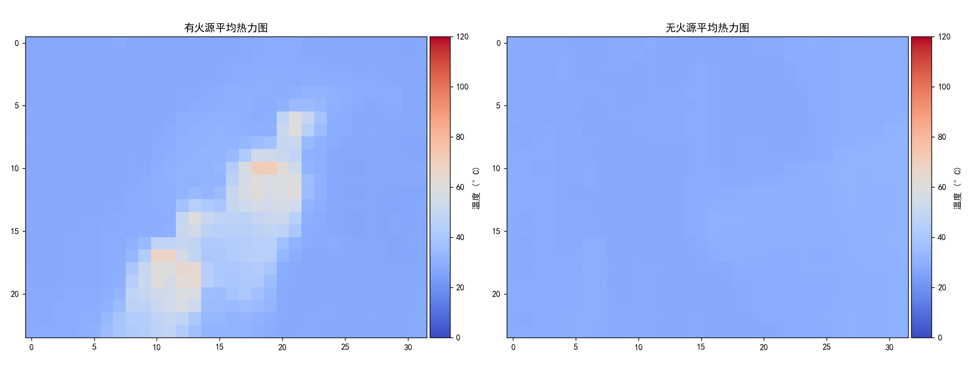
可以看出，有火源情况下的图像数据是有明显特征的，下面我们训练模型去分辨这些特征。

四、模型设计与训练

我们可以使用下面的代码对采集到的数据进行训练：

import os
os.environ['TF_ENABLE_ONEDNN_OPTS'] = '0'
import pandas as pd
import numpy as np
import tensorflow as tf
import matplotlib.pyplot as plt
from sklearn.model_selection import train_test_split
from sklearn.utils import shuffle

import matplotlib
matplotlib.rc("font",family='YouYuan')



# === 1. 读取和预处理数据 ===
df_1 = pd.read_csv('data/mlx90640_data_1.csv')
df_0 = pd.read_csv('data/mlx90640_data_0.csv')

data = pd.concat([df_1, df_0], ignore_index=True)
data = shuffle(data, random_state=42)

labels = data['label'].values.astype(np.int32)
features = data.drop(columns=['label']).values.astype(np.float32)

# 归一化 + reshape
features = features.reshape(-1, 24, 32, 1) / 100.0

X_train, X_test, y_train, y_test = train_test_split(
    features, labels, test_size=0.2, random_state=24
)

# === 2. 构建模型 ===
model = tf.keras.Sequential([
    tf.keras.Input(shape=(24, 32, 1)),  # 显式指定输入形状，避免警告
    tf.keras.layers.Conv2D(32, (3, 3), activation='relu'),
    tf.keras.layers.MaxPooling2D((2, 2)),
    tf.keras.layers.Conv2D(64, (3, 3), activation='relu'),
    tf.keras.layers.MaxPooling2D((2, 2)),
    tf.keras.layers.Flatten(),
    tf.keras.layers.Dense(64, activation='relu'),
    tf.keras.layers.Dense(1, activation='sigmoid')  # 二分类，sigmoid 输出概率
])


model.compile(optimizer='adam',
              loss='binary_crossentropy',
              metrics=['accuracy'])

# === 3. 训练模型并保存训练过程历史 ===
history = model.fit(X_train, y_train,
                    epochs=10,
                    batch_size=32,
                    validation_split=0.1)

# === 4. 可视化训练过程 ===
plt.figure(figsize=(12, 4))

# Loss
plt.subplot(1, 2, 1)
plt.plot(history.history['loss'], label='训练损失')
plt.plot(history.history['val_loss'], label='验证损失')
plt.title('损失曲线')
plt.xlabel('Epoch')
plt.ylabel('Loss')
plt.legend()

# Accuracy
plt.subplot(1, 2, 2)
plt.plot(history.history['accuracy'], label='训练准确率')
plt.plot(history.history['val_accuracy'], label='验证准确率')
plt.title('准确率曲线')
plt.xlabel('Epoch')
plt.ylabel('Accuracy')
plt.legend()

plt.tight_layout()
plt.show()

# === 5. 保存模型 ===
model.save('thermal_classifier_model.keras')
print("✅ 模型已保存为 thermal_classifier_model.keras")

# === 6. 评估模型 ===
test_loss, test_acc = model.evaluate(X_test, y_test)
print(f'🧪 测试准确率：{test_acc:.4f}')

# === 7. 加载模型并进行预测（多个样本） ===
# 从测试集中随机选择8个样本
random_indices = np.random.choice(len(X_test), 8, replace=False)
sample_images = X_test[random_indices]
true_labels = y_test[random_indices]

loaded_model = tf.keras.models.load_model('thermal_classifier_model.keras')
predictions = loaded_model.predict(sample_images, verbose=0)
pred_labels = (predictions > 0.5).astype(int).flatten()

# === 8. 显示这些热图 ===
plt.figure(figsize=(20, 10))

# 显示归一化后的图
for i in range(8):
    plt.subplot(2, 4, i+1)
    im = plt.imshow(sample_images[i].reshape(24, 32), cmap='coolwarm', 
                   interpolation='nearest', vmin=0, vmax=1)
    plt.colorbar(label='归一化温度')
    plt.title(f'样本 {i+1}\n实际: {true_labels[i]}, 预测: {pred_labels[i]}\n(概率: {predictions[i][0]:.2f})')

plt.tight_layout()
plt.show()

# 打印预测结果统计
print("\n=== 预测结果统计 ===")
correct = np.sum(pred_labels == true_labels)
print(f"✅ 正确预测数: {correct}/8 ({correct/8*100:.1f}%)")

这段代码实现了一个用于热成像图像二分类的完整深度学习流程：它首先读取并预处理两个类别的 MLX90640 热成像数据，将图像归一化并重塑为适合卷积神经网络的格式，然后构建了一个包含两层卷积和池化的简单 CNN 模型，使用交叉熵损失进行训练，并通过训练集和验证集观察模型表现。模型训练完成后被保存，并在测试集上进行了评估。最后，随机选取部分测试图像进行预测与可视化展示，同时统计预测准确率，验证模型实际分类效果。

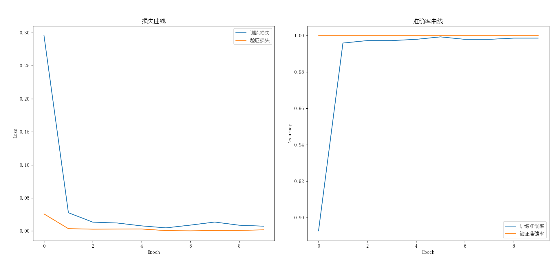
下面是模型训练过程中的损失曲线和准确率曲线：

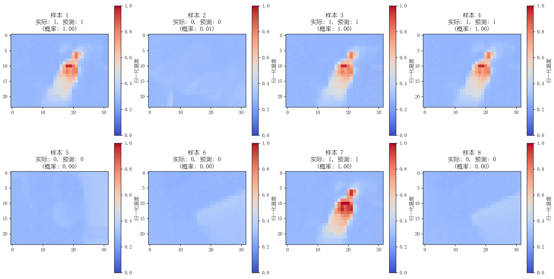
下面是使用训练的模型进行8个样本的预测，可以看到效果还可以：

经过训练我们得到了模型thermal_classifier_model.keras 接下来需要将模型转换为转换为TensorFlow Lite模型，使我们能将模型存放到嵌入式设备中去，可以使用下面的脚本：

import os
os.environ['TF_ENABLE_ONEDNN_OPTS'] = '0'
import tensorflow as tf

# Function: Convert some hex value into an array for C programming
def hex_to_c_array(hex_data, var_name):
    c_str = ''
    # Create header guard
    c_str += '#ifndef ' + var_name.upper() + '_H\n'
    c_str += '#define ' + var_name.upper() + '_H\n\n'
    # Add array length at top of file
    c_str += '\nunsigned int ' + var_name + '_len = ' + str(len(hex_data)) + ';\n'
    # Declare C variable
    c_str += 'unsigned char ' + var_name + '[] = {'
    hex_array = []
    for i, val in enumerate(hex_data):
        # Construct string from hex
        hex_str = format(val, '#04x')
        # Add formatting so each line stays within 80 characters
        if (i + 1) < len(hex_data):
            hex_str += ','
        if (i + 1) % 12 == 0:
            hex_str += '\n '
        hex_array.append(hex_str)
    # Add closing brace
    c_str += '\n ' + format(' '.join(hex_array)) + '\n};\n\n'
    # Close out header guard
    c_str += '#endif //' + var_name.upper() + '_H'
    return c_str


# 加载已保存的Keras模型
model = tf.keras.models.load_model('thermal_classifier_model.keras')

# 转换为TensorFlow Lite模型
converter = tf.lite.TFLiteConverter.from_keras_model(model)
converter.optimizations = [tf.lite.Optimize.DEFAULT]  # 如果想压缩模型可打开
tflite_model = converter.convert()

# 保存TensorFlow Lite模型
with open('thermal_classifier_model.tflite', 'wb') as f:
    f.write(tflite_model)
print("📦 已保存为 thermal_classifier_model.tflite")


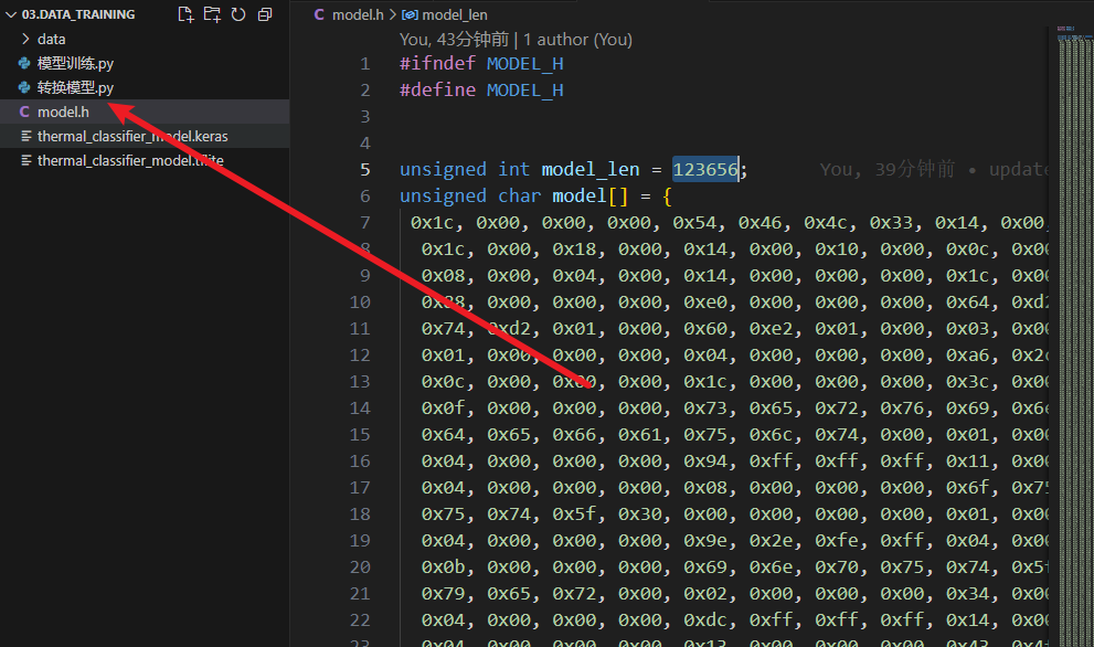
with open('model' + '.h', 'w') as file:
    file.write(hex_to_c_array(tflite_model, 'g_model'))

转换后我们可以得到模型文件：model.h 如果在文本编辑器中打开该文件，它应该看起来像一个标准的C头文件，顶部定义了模型长度，然后是一个巨大的字节数组。如下：

五、模型部署到 ESP32

预览模型：

可以使用 Netron 查看模型的图形界面。运行 Netron网站并使用它打开 thermal_classifier_model.tflite 文件。可以点击各个层以获取更多关于它们的详细信息，例如输入/输出张量形状和数据类型。

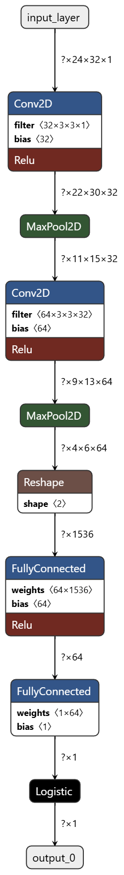
可以看到模型接收的是尺寸为 24x32 的单通道热图像，输出为0（有火焰），1（无火焰）两种标签分类。

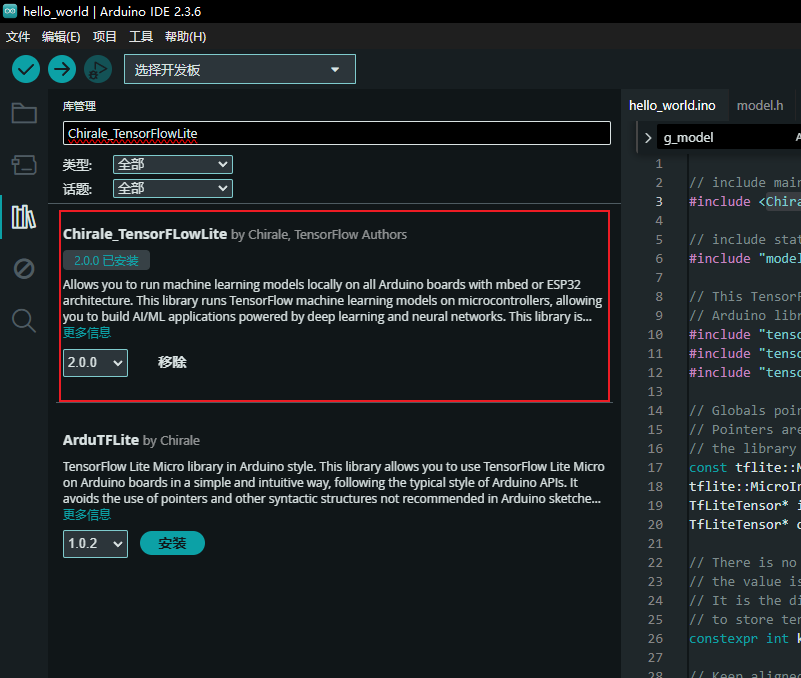
安装支持库：

为了在arduino上调用模型，我们需要使用Chirale_TensorFlowLite这个库：

使用下面的代码去调用模型：

#include <Wire.h>
#include <Adafruit_MLX90640.h>
#include <Chirale_TensorFlowLite.h>
#include "model.h"
#include "tensorflow/lite/micro/all_ops_resolver.h"
#include "tensorflow/lite/micro/micro_interpreter.h"
#include "tensorflow/lite/schema/schema_generated.h"

constexpr uint8_t SDA_PIN = 8;
constexpr uint8_t SCL_PIN = 7;
#define MLX_ADDR 0x33

constexpr int kTensorArenaSize = 110000; // 根据模型适当增大
alignas(16) uint8_t tensor_arena[kTensorArenaSize];

Adafruit_MLX90640 mlx;
float frame[32 * 24];

// TFLite组件指针
const tflite::Model *model = nullptr;
tflite::MicroInterpreter *interpreter = nullptr;
TfLiteTensor *input = nullptr;
TfLiteTensor *output = nullptr;

float scale;
int zero_point;

void setup()
{
  Serial.begin(115200);
  delay(50);

  Wire.begin(SDA_PIN, SCL_PIN);
  Wire.setClock(100000);

  Serial.println("初始化热成像传感器...");
  if (!mlx.begin(MLX_ADDR, &Wire))
  {
    Serial.println("传感器未连接！");
    while (1)
      delay(1000);
  }
  mlx.setMode(MLX90640_CHESS);
  mlx.setResolution(MLX90640_ADC_18BIT);
  mlx.setRefreshRate(MLX90640_2_HZ);

  Serial.println("初始化 TFLite Micro...");
  model = tflite::GetModel(g_model);
  if (model->version() != TFLITE_SCHEMA_VERSION)
  {
    Serial.println("模型与库版本不兼容！");
    while (1)
      ;
  }

  static tflite::AllOpsResolver resolver;
  static tflite::MicroInterpreter static_interpreter(model, resolver, tensor_arena, kTensorArenaSize);
  interpreter = &static_interpreter;

  if (interpreter->AllocateTensors() != kTfLiteOk)
  {
    Serial.println("张量内存分配失败！");
    while (1)
      ;
  }

  input = interpreter->input(0);

  scale = input->params.scale;
  zero_point = input->params.zero_point;



  output = interpreter->output(0);

  Serial.println("系统初始化完成，开始推理...");
}

void loop()
{
  if (mlx.getFrame(frame) != 0)
  {
    Serial.println("读取热图失败，跳过本帧");
    delay(100);
    return;
  }

  // 转换并填充输入张量（int8）
  for (int i = 0; i < 768; i++)
  {
    float val = frame[i];
    int8_t q = val / scale + zero_point;
    input->data.int8[i] = q;
  }

  // 执行推理
  if (interpreter->Invoke() != kTfLiteOk)
  {
    Serial.println("推理失败！");
    return;
  }

  // 读取输出并解码
  int8_t result = output->data.int8[0];
  float score = (result - output->params.zero_point) * output->params.scale * 2;

  Serial.print("得分：");
  Serial.print(score);

  Serial.print("推理结果：");
  if (score >= 0.6)
  {
    Serial.println("🔥 检测到火焰");
  }
  else
  {
    Serial.println("✅ 无火焰");
  }
  delay(1000);
}

这段代码完成了一个基于热成像识别火焰的嵌入式推理系统，核心功能包括以下几个部分：

• 初始化外设：使用 I2C 接口初始化 MLX90640 热成像传感器，设置其工作模式为 CHESS 模式、分辨率为 18bit、刷新率为 2Hz，确保稳定读取 32×24 个温度点的图像数据。
• 加载 TFLite Micro 模型：将量化后的 int8 模型通过 TensorFlow Lite Micro 加载至内存中，并配置推理引擎，包括张量分配、操作解析器初始化等。
• 输入量化处理：将读取到的每个浮点温度值按模型输入张量的 scale 和 zero_point 量化为 int8 类型，并填入输入张量中。
• 执行推理：调用 interpreter->Invoke() 执行模型推理，获取输出张量中的预测结果。
• 输出反量化与判断：将 int8 类型的输出反量化为浮点得分，并乘以 2（这是你自定义的扩展系数，用于调整阈值感知范围）。若得分大于 0.6，即认为检测到火焰，否则判断为无火焰。
• 串口输出结果：通过串口打印输出推理得分和判断结果，用于调试或后续联动使用。

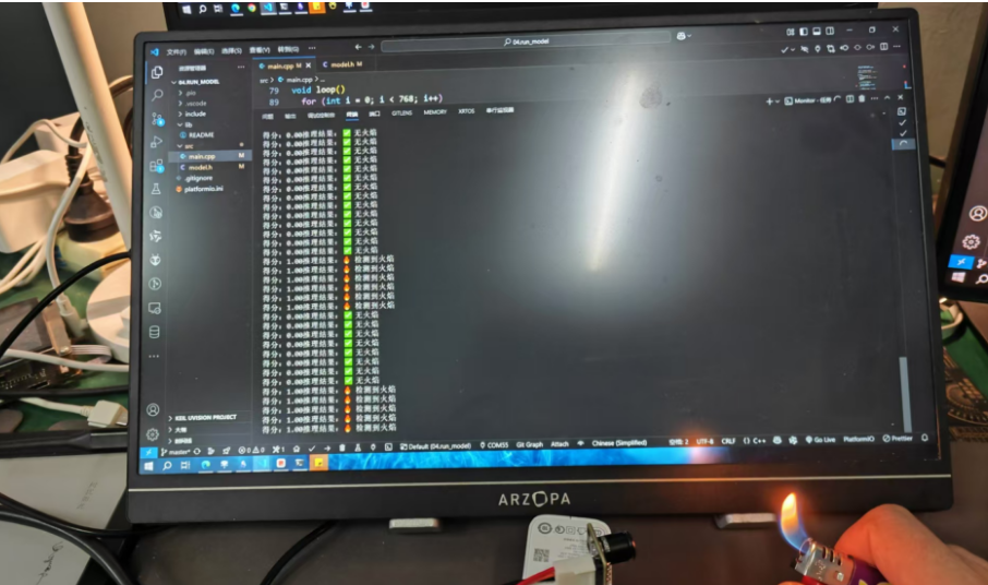
六、设备联动与效果展示

代码运行效果如下，可以完美识别到火焰信息。

七、遇到的问题与解决方案

运行过程中出现：

得分：-0.00推理结果：✅ 无火焰
得分：-0.00推理结果：✅ 无火焰
得分：-0.00推理结果：✅ 无火焰
得分：-0.00推理结果：✅ 无火焰
得分：-0.00推理结果：✅ 无火焰
得分：-0.00推理结果：✅ 无火焰
得分：-0.00推理结果：✅ 无火焰
得分：-0.00推理结果：✅ 无火焰
得分：-0.00推理结果：✅ 无火焰
得分：-0.00推理结果：✅ 无火焰
得分：-0.00推理结果：✅ 无火焰

进一步发现模型数据输入异常：

  // 转换并填充输入张量（int8）
  for (int i = 0; i < 768; i++)
  {
    float val = frame[i];
    int8_t q = val / scale + zero_point;
    input->data.int8[i] = q;
  }

异常如下：如果相同的 val 对应的 q 差别极大

al:31.75
q:-97
val:32.10
q:-8
val:31.91
q:-55
val:31.97
q:-40
val:31.79
q:-86
val:31.77
q:-90
val:31.80

最后调试发现：

scale:0.00zero_point:0val:31.68
q:-114
scale:0.00zero_point:0val:30.50
q:96

input->params.scale == 0.00，这是严重错误！

int8_t q = val / input->params.scale + input->params.zero_point;

除以 0 的行为，虽然在 C++ 中可能不会 crash，但会导致 量化值乱跳，完全错误的结果（如 q=96, -114, 125...）。

进一步检查是模型量化信息导致：

输入数据类型: <class 'numpy.int8'>        
输入量化信息: (0.003921534400433302, -128)
输出数据类型: <class 'numpy.int8'>        
输出量化信息: (0.00390625, -128)

量化参数中的 scale 值太小（约 0.0039），导致在单片机端反量化时几乎都为 0

最终解决办法为去除模型训练时的数据归一化，使用温度原始值进行训练。

八、参考附录

1. https://www.bilibili.com/video/BV1EK4y177Sn
2. https://www.bilibili.com/video/BV1uX8veJEGi
3. Intro to TinyML Part 1: Training a Model for Arduino in TensorFlow (digikey.com)
4. Intro to TinyML Part 2: Deploying a TensorFlow Lite Model to Arduino (digikey.com)
5. https://blog.tensorflow.org/2019/11/how-to-get-started-with-machine.html?hl=zh-cn